Features and Usages
Spreadsheet User Interface Overview
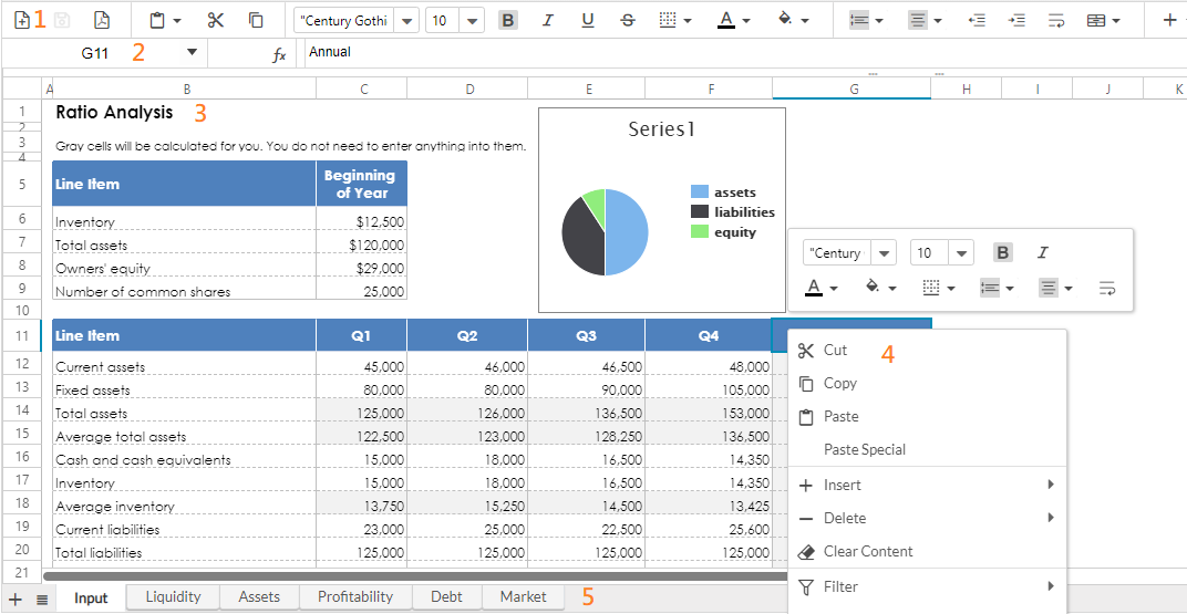
Above is Keikai spreadsheet’s user interface, each section is introduced as follows:
1.Toolbar
The toolbar contains the commonly-used features including font size, family, alignment, border, background color, font color, merge (and unmerge), sorting, auto filter, protection, grid line visibility and to insert charts, images, and hyperlinks.
The 2 buttons: Save Book, and Export to PDF are disabled by default because they highly depend on your requirements. You have to implement the logic by yourself, please read Toolbar Customization.
2. Formula bar
It displays cell value or formula of the current selected cell. It can also be used for entering or editing a formula or cell value.
3. Sheet Area
It displays the content of current selected sheet, this is also the area where users normally work with.
4. Context menu
A context menu is displayed when you right click on a cell, a column header, or a row header. It contains most options of the toolbar and works like a shortcut.
5. Sheet bar
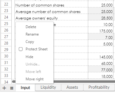
Sheet bar displays a list of all sheets in this book. You can navigate to any sheet by clicking on it. You can add a sheet by clicking the + button on the left. If you right click on the sheet bar it pops up a context menu, and allows you to perform sheet operations.
The hamburger menu next to the + icon is the sheet navigation button. It allows users to switch a sheet via a sheet name list.
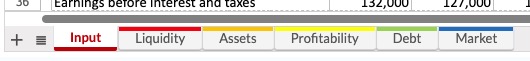
Tab Color
since 5.2.0
Tab color is imported and rendered.
Supported Hotkeys
Hotkey |
Action |
|---|---|
CTRL+B |
bold |
CTRL+C |
copy |
CTRL+I |
italic |
CTRL+U |
underline |
CTRL+V |
paste |
CTRL+X |
cut |
CTRL+Y (EE only) |
redo |
CTRL+Z (EE only) |
undo |
Delete |
clear content |
Esc |
clear copy/cut clipboard |
CTRL+ARROW KEY |
moves the selection box to the edge of the current data region in a sheet. |
Text Style
bold, italic, underline, strikeout, color, background color, vertical/horizontal alignment, indent, wrap
since 5.3.0
double underline
- Not supported for IE 11 or below
Wrap Text
When wrap text is enabled, keikai wraps a cell’s text into multiple lines according to the column width.
Besides, keikai will automatically resize a row height to completely display the wrapped text. So keikai will increase the height when there are more texts and reduce the height when removing the text. Note that wrap text, same as Excel’s wrap text, doesn’t apply to the following cases:
- a row with custom height
- a merged cell
Charts
The charts in Keikai sheet is rendered by another ZK product called ZK Charts. When you hover your mouse pointer over the charts, it will show related info in a tooltip.
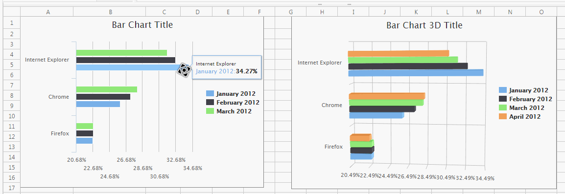
The supported elements and options for a chart in a xlsx file are listed as follows:
- Chart Title
- Primary/Secondary Axes
- Primary Major Horizontal/Vertical Gridlines
- Legend (position)
- Data Series Color
Limitations:
- Ignore unsupported elements and options during importing and render a chart with built-in setting.
- Convert a theme color of a data series to a fixed color code and export it as the fixed color.
- When exporting to a PDF file, combination chart and sparklines are not supported, the color will not be consistent with the color you see in a browser. (Because Keikai exports charts to PDF with jFreeChart.)
Dynamic title from formula
since 5.8.0
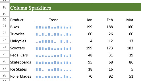
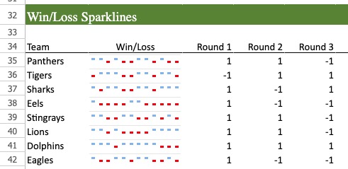
Sparklines
since 5.3.0
Sparklines is a chart that fits in one cell. There 3 types of sparklines supported:
Line
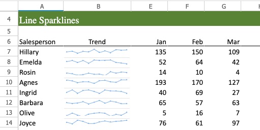
Column
Win-Loss
Limitation
- It doesn’t resize itself when you resize the cell.
- Render with built-in color (ignore color when importing).
- Export it with built-in color.
Combo Chart
since 7.0.0 Keikai 7.0.0 supports formula declaration for charts title and legends
A combination chart is a chart that displays 2 types of chart in a single chart.
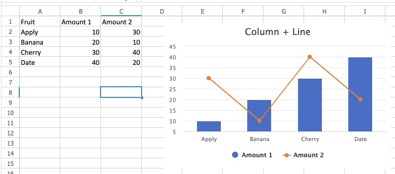
Empty Cell
since 5.8.0 Keikai can show an empty cell as zero or gap depending on how you configure each chart in Excel.
![]()
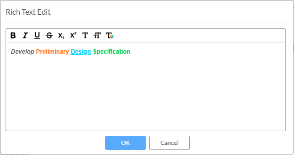
Rich Text Editing
You can apply multiple styles to a same cell by using the rich text editor. To open a rich-text editor, right click a cell and select “Right Text Edit” in the context menu. See more details.
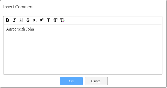
Comment
To insert/edit/delete a comment, right click a cell and select corresponding item in the context menu.
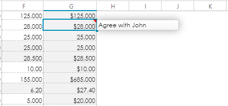
Show comment
Support Different Zoom Levels
You can view Keikai in different browser zoom levels.
Support Locale Currencies
Keikai can display different currency symbols for different local such as $, ¥, ₩, €, and HKD in a cell in the currency format.
[$-409]0.00: 409 is a locale ID in hexadecimal, please see Windows Locale Codes
Localize A Number/Formula Input
Keikai also accepts ,(comma) or .(dot) as the decimal point for decimal numbers.
Smart Input
When you enter a text in a cell with the default format (General), keikai will try to identify the input text as a number or a date value with the supported patterns below. If keikai can’t identify the input text as a number/date, then it just keep the input as it is.
For example, if you enter $123 in a cell, keikai converts it as a number cell and apply a currency format on it instead of keeping it as a text $123. You can do math operation with a number but not with a text.
Independent of Number Format
The smart input pattern determines how you enter a date value. That is independent of a cell’s number format that determines how to display a date value. When entering the edit mode (pressing F2 or double clicking a cell), keikai switches to one of the supported input patterns instead of the number format.
JVM Option
If you run JDK 9 or above, this feature needs a corresponding JVM option to work properly.
Locale Dependent
Under different locale, keikai supports different input patter, see how Keikai/ZK determines the current locale.
Supported Number Pattern
1,234,567, $123456, ($123456), ($1,234,567), 1.2% or 123456E10.
Supported Date Pattern
d-mmm-yyd-mmmmmm-yym/d/yyyym/d/yyyy h:mm
Smart Percentage Scaling
When a cell is already formatted as Percentage, Keikai applies “Smart Percentage Scaling” to numeric inputs to maintain consistency with Excel’s behavior. This logic follows a 1.0 Threshold:
- Input ≥ 1.0: The value is treated as the percentage itself. For example, entering
1results in1%. - Input < 1.0: The value is treated as a decimal fraction and is multiplied by 100. For example, entering
.1results in10%.
This behavior ensures that both fractional and whole-number percentage inputs are handled intuitively. Keikai also supports signed decimal inputs such as -.15 (which becomes -15%) or .15.
Date Format
Some date formats in Keikai are regional (starting with an asterisk, *, same as Excel ) and some are international (without an asterisk *).
Regional ones will change its displaying format according to the system locale, but international ones won’t change. Please refer to Microsoft Office Support - Format a date the way you want.
- If you run JDK 9 or above, this feature needs a corresponding JVM option to work.
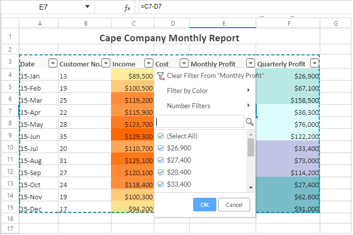
Conditional Formatting
Keikai can display conditional formatting you specify in an Excel file. This feature allows you to highlight cells with the given conditions. In the case below, the values in the “Income” column has conditional formatting enabled:
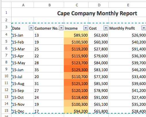
- Modifying conditional formatting in Keikai UI or API is not supported yet.
Named Range
Keikai can read a named range from an xlsx file, so you can specify a named range in a formula like =SUM(source). To create a named range, please reference Range::createName.
Copy & Paste
We recommend you to copy and paste with Ctrl+c and Ctrl+v which works in all cases rather than clicking “paste” button on the toolbar and “paste” item on the context menu. Copy a cell with a multi-line text and paste to Keikai cell is supported.
Inside One Spreadsheet
- Such copy-paste works with Ctrl+c and Ctrl+v, the toolbar, and context menu.
- Keikai has full information at both server and client side, so such copy-paste can retain all cell information including styles, formula, format, and data validation.
- If you copy a whole column/row, Keikai also copies its width and height. But if you are only copying one or multiple cells, Keikai won’t copy the width and height.
- When copy highlight is still active, it copies the highlighted cells, not from the system clipboard. You need to cancel the copy highlight first, then you can paste from a system clipboard.
Between 2 Keikai components
- Copy-paste cell data between 2 Keikai components also rely on the system clipboard, so it’s similar to copy/paste between Keikai and Excel – only pure text is copied.
- If you want to copy a whole sheet to another Keikai component,
please call
Range.cloneSheetFrom. It can clone a sheet from anotherBookobject and is more performant.
Between Keikai and Other Applications like Excel
- Such copy-paste will only work with Ctrl+C and Ctrl+V. The toolbar or context menu “Paste” button only works for copying cells within the same Keikai component and will not work across different applications.
- Such copy-paste is an action between 2 applications (Excel and browser) through a system clipboard. Currently, Keikai only extract text content from a system clipboard, so this copy-paste only pastes “pure text” without any styles.
- For example, a cell in Excel has a formula
=sum(1,2)which is3. If you copy this cell and paste it into Keikai, the cell in Keikai gets the calculated3as its value. Just like you type3in a Keikai cell. - If you enter edit mode in Excel and select the text
=sum(1,2)and copy it, and then paste it to a cell in Keikai, Keikai will get the formula, just like you typed a formula into the Keikai cell. - If you copy cells in Keikai, then copy cells in Excel, when you paste cells (
ctrl+v), Keikai will paste cells in Keikai first since Keikai is still in its copy mode. You need to exit the copy mode (by pressingEsckey or editing any cell), then you can paste the cells from Excel.
Paste Special
In addition to standard pasting, Spreadsheet also provides custom pasting options in the toolbar.
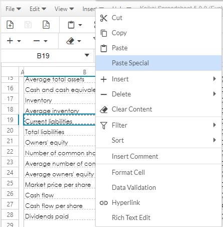
You can select “Paste Special” to access all available pasting options in the dialog.

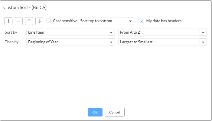
Custom Sort
With the “Ascending” and “Descending” function you can sort data by only one column, with “Custom sort” you can sort data by multiple columns.
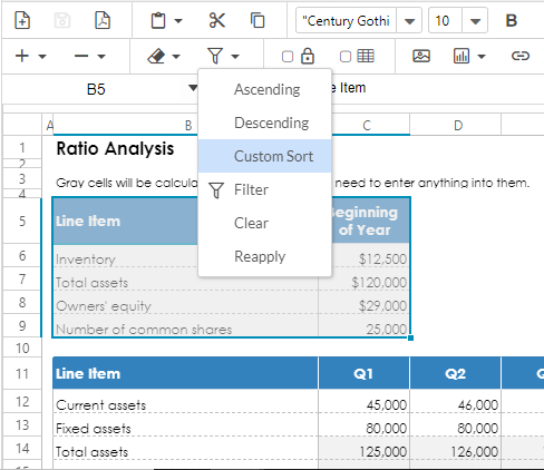
After selecting “Custom sort” on the toolbar, a dialog appears. You can add sorting criteria up to 3 columns. If your data includes column header, make sure the “My data has headers” option is checked.
Auto Fill
Auto fill is a handy feature to fill cells with data in a particular pattern based on selected cells. Text will be copied and numbers and dates will be increased (or decreased) as you drag through.
To use this, select one or more cells and drag the fill handle across or down the cells that you want to fill.
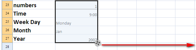
Fill cells by dragging right, left, up, or down.
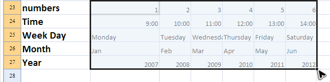
The supported cell content are number, weekday (full/short), month (full/short), and timestamp.
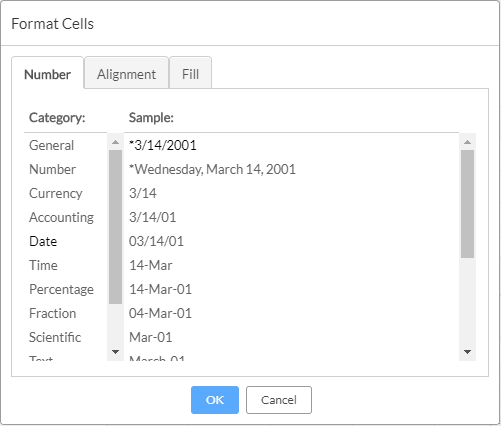
Format Cell
The Format Cell option is in the context menu. It provides 10 different categories with a total of 47 formats to apply to the cells.
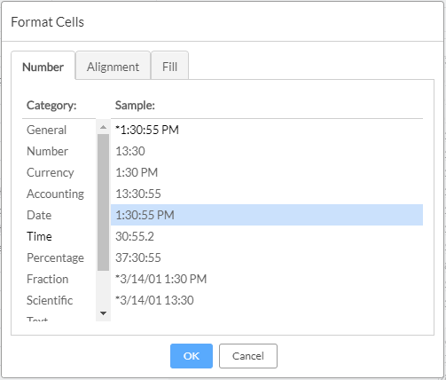
Locale-Aware Date and Time Formats
since 6.3.0
The items marked with * in the Format Cells dialog are locale-aware. Their format patterns and preview labels are dynamically determined by the browser language settings. Please see Locale-Aware Date and Time Formats.
Sheet Protection
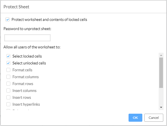
If you enable “Protect Sheet” against a sheet in Excel, Keikai will keep this setting when reading the Excel file, hence, when you edit a protected sheet, you will see an alert message telling you that the sheet is being protected.
When a sheet is under protection, users can only edit unlocked cells. You can specify which actions are allowed for unlocked cells.
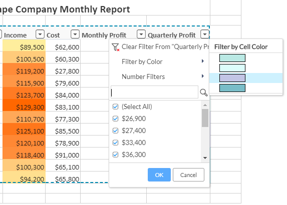
Filters
A filter can help you screen out data and work with a subset of data in a range of cells without moving or deleting them.
When you click on the filter icon, there are 3 menu items: Filter, Clear, and Reapply relating to the filter.
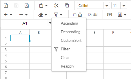
Click the funnel-like “Filter” icon to enable/disable filters. When filters are enabled, a drop-down icon will show up in the first row of each column. If you click the drop-down icon, a list of values will appear and you can select from the list as the filtering criteria to apply to your data.
After you select some values, click OK and Spreadsheet will filter those data with selected values. Only the rows with matching criteria will be displayed while others will be hidden.
You can also filter by multiple columns. Filters are additive, which means that each filter is based on the existing filters and further reduces the subset of data.
Click “Clear” removes all applied criteria and displays all data available.
If you added a new data row, you should click “Reapply”. The drop-down list will then update its values to take into account the newly added data.
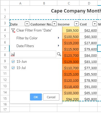
Filter by search
When you enter text in the search box of the filter, it will instantly list and select all matched cell values. Press “Enter”. Then, Keikai will filter the rows with those matched values, no matter you select those values or not.
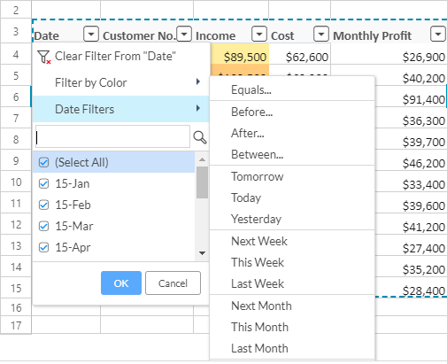
Filter Types
Keikai supports number filter, color filter, date filter, and text filter.
Auto-detect Filtering Range
- When users select just 1 cell, find the largest range surrounded by blank cells
- When users select an area (multiple cells)
- If the non-blank cell range is smaller than the area, shrink to the non-blank cell range
- If the non-blank cell range is larger than the area, only extends its bottom boundary, keep the left, top and right boundary as the same as the selection
- When users select the whole rows such as
5:10, find the continuous non-blank cell range between row 5 and 10 - When users apply a filter, Keikai will detect non-blank cells again to change the filtering range.
Data Validation
Spreadsheet can read Excel data validation settings including validation criteria of lists, numbers, decimals, dates, or time.
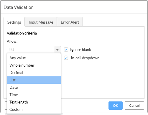
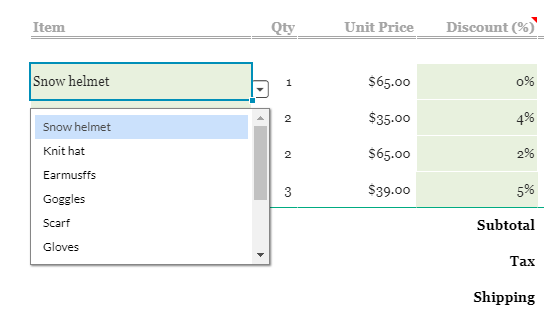
If the validation criteria is a list, the cell will display a drop-down arrow. You can click the icon to select available values.
When you click on the cell with validation, the input message you set will be displayed automatically.
If your input violates validation criteria, an error alert will pop up.
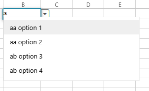
Items Filtering (Type to Narrow Items)
since 6.1.0 As you type in the dropdown field, the list instantly filters to show only matching items. This makes it easy to quickly find and select the desired value from large lists.
Keyboard Support
since 6.1.0 Press Alt + Down to open the dropdown, then use the arrow keys or mouse to navigate items.
List
There are 2 ways to specify a list criteria:
List of values
Specify the source field with comma-sperate values: 30 days,60 days
Named Range
Specify a named range that contains a list of items: =PRODUCT_LIST
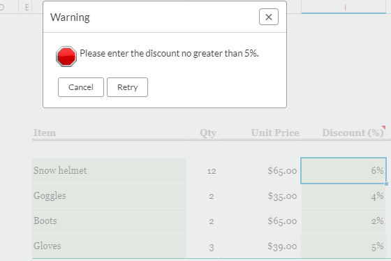
Alert
There are 3 types of alerts and each of them has a different icon in the dialog:
- For an error alert (red icon), you can retry and enter again or cancel to revert back to the original value.
- For a warning alert (yellow icon), you can click “Yes” to accept the invalid input, or, “No” to edit the invalid input, or “Cancel” to remove the invalid input.
- For an information alert (blue icon), you can click “OK” to accept the invalid value or “Cancel” to reject it.
Limitation:
- custom validation is not supported yet.
- Validation lists using a formula referencing a different sheet are not supported due to Excel data structure. To use data from a different sheet as source for a validation list, you must create a named range containing the data, and use that named range as the validation data source.
Table
Keikai supports to load an Excel table. If your add (or remove) rows/columns to a table, keikai will automatically keep the color theme of cells. You don’t need to set background and borders by yourselves.
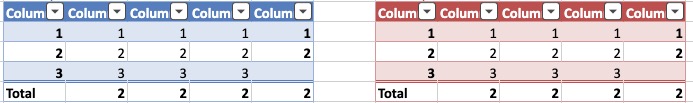
Limitation
- Regarding table colors, keikai only supports Office2007-2010 color. If you choose an unsupported color in Excel, the color will be turned to the supported color. So the color will look different in Keikai.
AutoFit
Please see AutoFit.
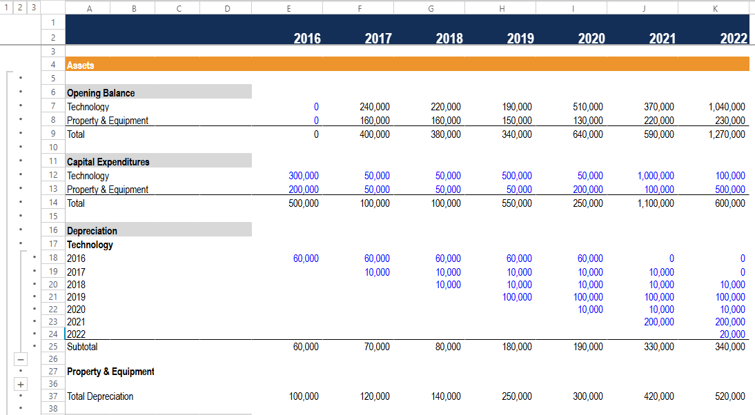
Group
Keikai allows users to organize rows or columns into collapsible sections. This feature helps you group and collapse related rows or columns, making it easier to navigate large datasets like financial reports or task lists. With just a few clicks, you can group related rows or columns and easily expand or collapse them to show or hide details.
Macro-Enabled Workbook (VBA)
since 7.0.0
Keikai can import and export macro-enabled xlsm workbooks while preserving their VBA macro project.
- When importing an xlsm file, Keikai keeps the VBA macro project (
xl/vbaProject.bin) intact byte-for-byte;Book.getType()returnsBookType.XLSMandBook.getVbaProject()returns the macro binary. - When exporting, the xlsx exporter automatically writes a macro-enabled workbook (with the
application/vnd.ms-excel.sheet.macroEnabled.main+xmlcontent type) whenever the book carries a VBA project, so the macros survive a round-trip and remain runnable in Excel.
For details and code examples, see Import a Macro-Enabled Workbook and Export to Excel.
Limitation
- Keikai keeps the VBA macro project as-is but does not parse, run, or edit the macro code.
- VBA macros are only supported for the xlsx/xlsm format; the deprecated xls (BIFF8) format cannot carry an OOXML VBA part.
Excel Export Options
since 7.0.0
Keikai supports export-time customization for xlsx/xlsm files through ExportOptions.
You can choose how formula cells are written to the exported workbook: keep formulas, blank formula cells, or export calculated values only. You can also apply a per-cell rule, for example exporting custom formula functions as values only so Excel does not try to parse formulas it does not support.
ExportOptions can also skip comments or hyperlinks in the exported file. These options affect only the exported workbook and do not mutate the source book model.
For details and code examples, see Export to Excel.